Conventional metadynamics¶

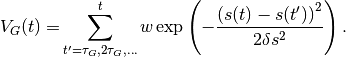
The metadynamics method is implemented according to the original paper by Laio and Parrinello (A. Laio, M. Parrinello, Proc. Nat. Acad. Sci. USA 99 (20), 12562 (2002)). In this method, one or multiple collective variables (CVs) $s(t)$ are used to add Gaussians of fixed height $w$ and width $\delta s$ every $\tau_G$ steps to a history-dependent bias potential of the form

$V_{G}(t)= &\sum_{t'=\tau_{G},2\tau_{G},\ldots}^{t}w\exp\left(-\frac{\left(s(t)-s(t')\right)^{2}}{2\delta s^{2}}\right).$

Input preparation¶

As a preparation, open the GUI application and fill out the forms in the Molecular Dynamics tab to perform a MD simulation of 1,3-butadiene at constant temperature of 300 K for several ps of equilibration (butadiene.xyz). Then run the simulation and create a new folder for the metadynamics run. When you start the GUI application in the new folder, choose Import from the File menu to import the configuration of the equilibration. You want to use the coordinates and velocities from the last step of the equilibration, so take the bottom option for the generation of initial conditions and specify the path to the previous results. The last step of the dynamics is taken, if no other value is given in the step form. Finally, switch to the Metadynamics tab and check the Do metadynamics box.

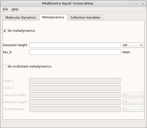
Enter the Gaussian height and the number of time steps $\tau_{G}$ that should pass between the addition of two Gaussians. The definition of collective variables (CV) is done in the third tab.

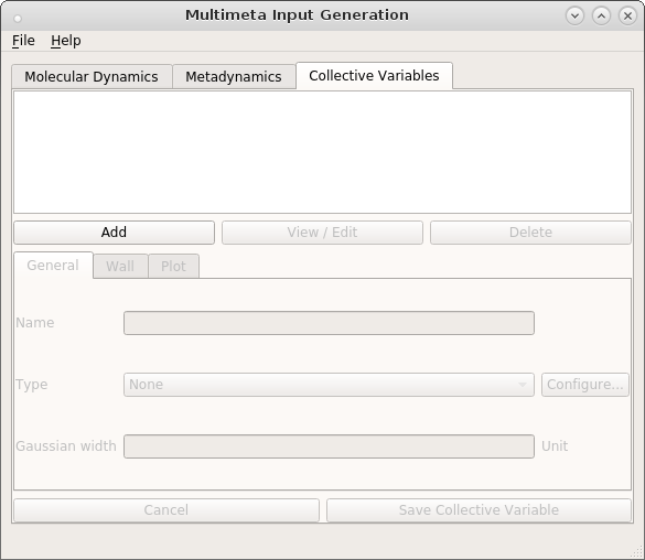
Click Add to create a new CV.

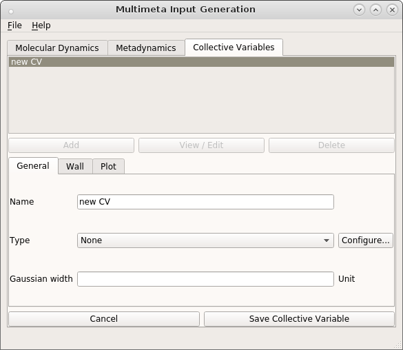
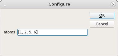
Choose a name and a type for the CV, in our case we want to describe the transition between the cis- and trans-forms of butadiene, so choose torsion from the drop-down menu. The atom indices that define the torsion angles are provided as a python list in the Configure… dialog.

The last thing to be entered is the Gaussian width. We can choose a value of 10 degrees as a starting point. After saving the CV, you can edit and delete it again or add another one. You can download the complete meta-config.json file, if you have any problems.

Run metadynamics¶

Start the metadynamics run just as a normal MD run:

metaFALCON run

Analyze results¶

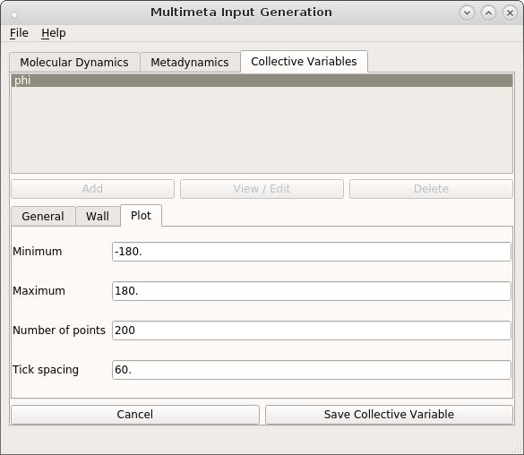
A plot of the current metadynamics potential is obtained during or after the dynamics run with the reconstruct command line tool. In this program, the potential is reconstructed by summation of all Gaussians on a grid of CV values. The grid is most easily adjusted in the plot tab of the CV editing function of the GUI application.

Use

metaFALCON reconstruct --help

for an overview of all options of the reconstruction utility. For example, if you want to animate the potential evolution along the addition of Gaussians instead of the last frame only, the animate option is helpful:

metaFALCON reconstruct --animate

Reconstruction works well for metadynamics with one or two collective variables. For higher dimensions, the grid and $V_G$ values are also saved as binary numpy array files, but it is not possible to obtain a potential plot without further processing.